机器学习——RNN系列网络
引言
授课过程中,对于RNN、GRU和LSTM,发现有一些难点需要梳理。调用pytorch中的torch.nn库尽管方便,但没法深刻理解公式和代码的对应关系。因此,写一篇博客记录一下这些网络的原理和手搓实现过程。
RNN

简单的MLP网络没法利用序列前后的信息,并且参数量很大。
RNN 通过引入“循环”结构,使得网络能够在处理当前输入时,利用之前步骤的信息。这种特性使其非常适合处理时间序列、文本、语音等具有顺序关系的数据,让模型具有短期记忆能力。
公式
隐藏层在时间t的更新公式:
$$
h_t = \sigma(W_{hx}\cdot x_t+W_{hh}\cdot h_{t-1} + b_h)
$$
其中$\sigma$是激活函数,tanh或ReLU。$x_t$是t时刻的输入,$h_t$是当前的隐藏状态
$h_{t−1}$是上一时刻的隐藏状态
输出层公式:
$$
y_t = W_{hy} \cdot h_t + b_y
$$
$y_t$是当前时刻的输出
RNN的隐藏状态$h_t$起到了记忆的作用。
对于一整个序列,图示如下:
pytorch实现
可使用pytorch封装的nn.RNN模块。
 1
 2
 3
 4
 5
 6
 7
 8
 9
10
11
|
class RNNModel(nn.Module):
    def __init__(self, input_dim, hidden_dim, output_dim=1, num_layers=1):
        super(RNNModel, self).__init__()
        self.rnn = nn.RNN(input_dim, hidden_dim, num_layers, batch_first=True)
        self.fc = nn.Linear(hidden_dim, output_dim)

    def forward(self, x):
        x, _ = self.rnn(x)
        x = x[:, -1, :]
        x = self.fc(x)
        return x
|
其实手搓一点都不难。熟练使用nn.Parameter,@或torch.matmul代表矩阵相乘,*代表逐元素相乘。其他都非常简单,照着公式写出来即可。
 1
 2
 3
 4
 5
 6
 7
 8
 9
10
11
12
13
14
15
16
17
18
19
20
21
22
23
24
25
26
27
28
29
|
class SimpleRNN(nn.Module):
    def __init__(self, input_dim, hidden_dim, output_dim=1):
        super(SimpleRNN, self).__init__()
        self.hidden_dim = hidden_dim
        # 定义每一层的权重和偏置
        self.W_xh = nn.Parameter(torch.randn(input_dim, hidden_dim))
        self.W_hh = nn.Parameter(torch.randn(hidden_dim, hidden_dim))
        self.b_h = nn.Parameter(torch.randn(hidden_dim))
        # 输出层
        self.fc = nn.Linear(hidden_dim, output_dim)

    def forward(self, x):
        # x 的形状: (batch_size, sequence_length, input_dim)
        batch_size, sequence_length, input_dim = x.size()
        # 初始化隐藏状态
        h = torch.zeros(batch_size, self.hidden_dim)
        # 遍历时间步

        # nn.RNN相当于做了这个循环
        for t in range(sequence_length):
            x_t = x[:, t, :]  # 当前时间步的输入 (batch_size, input_dim)
            h = torch.tanh(
                x_t @ self.W_xh) +
                h @ self.W_hh) +
                self.b_h
            ) # 与公式对应
        # 取最后一层的最后一个时间步的隐藏状态
        output = self.fc(h)
        return output
|
可以看到代码
1
|
h = torch.tanh(x_t @ self.W_xh + h @ self.W_hh + self.b_h)
|
和公式$h_t = \sigma(W_{hx}\cdot x_t+W_{hh}\cdot h_{t-1} + b_h)$严格对应。
LSTM
LSTM(Long Short-Term Memory)是一种经典的基于门控的循环神经网络。通过三个门和两个隐藏状态来完成长短期记忆。
遗忘门
$$
f_t = \sigma(W_f \cdot [h_{t-1}, x_t] + b_f)
$$
1
|
f_t = torch.sigmoid(h @ self.W_hf + x_t @ self.W_xf + self.b_f)
|
sigmoid函数将隐藏层和输入量拼接后变换到0-1之间,记作$f_t$。这个遗忘门用于控制$h_{t-1}的占比
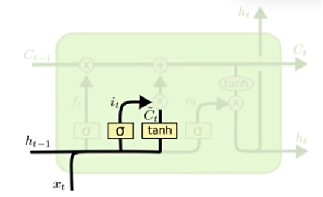
输入门
$$
i_t = \sigma(W_i \cdot [h_{t-1}, x_t] + b_i) \
\tilde{C}t = tanh(W_C \cdot [h{t-1}, x_t] + b_C)
$$
1
2
|
i_t = torch.sigmoid(h @ self.W_hi + x_t @ self.W_xi + self.b_i)
candidate_C = torch.tanh(h @ self.W_hC + x_t @ self.W_xC + self.b_C)
|
$i_t$代表输入门的权重
通过tanh映射到[-1, 1]之间,获得候选记忆细胞状态。
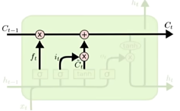
更新记忆细胞
$$
C_t = f_t\odot C_{t-1} + i_t \odot \tilde{C}_t
$$
1
|
C = f_t*C + i_t * candidate_C
|
用遗忘门权重$f_t$控制旧的细胞占比,用输入门权重控制$\tilde{C}_t$的权重占比。
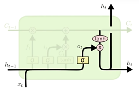
输出门
$$
o_t = \sigma(W_o\cdot [h_{t-1}, x_t] + b_o) \
h_t = o_t \odot tanh(C_t)
$$
1
2
|
o_t = torch.sigmoid(h @ self.W_ho + x_t @ self.W_xo + self.b_o)
h = o_t * torch.tanh(C)
|
控制输出量的权重
事实上,细胞状态C负责长期记忆,隐藏层h负责记忆短期记忆。所以LSTM就这样得名了。
pytorch实现
 1
 2
 3
 4
 5
 6
 7
 8
 9
10
11
12
|
class LSTMModel(nn.Module):
    def __init__(self, input_size, hidden_size, num_layers=1, output_size=1):
        super(LSTMModel, self).__init__()
        self.hidden_size = hidden_size
        self.num_layers = num_layers
        self.lstm = nn.LSTM(input_size, hidden_size, num_layers, batch_first=True)
        self.fc = nn.Linear(hidden_size, output_size)

    def forward(self, x):
        out, _ = self.lstm(x)
        out = self.fc(out[:, -1, :]) # 将最后一个隐藏层通过线性层变成结果
        return out
|
 1
 2
 3
 4
 5
 6
 7
 8
 9
10
11
12
13
14
15
16
17
18
19
20
21
22
23
24
25
26
27
28
29
30
31
32
33
34
35
36
37
38
39
40
41
42
43
44
45
46
47
48
|
class SimpleLSTM(nn.Module):
    def __init__(self, input_dim, hidden_dim, output_dim=1):
        super(SimpleLSTM, self).__init__()
        self.hidden_dim = hidden_dim
        # 定义每一层的权重和偏置
        self.W_xf = nn.Parameter(torch.randn(input_dim, hidden_dim))
        self.W_hf = nn.Parameter(torch.randn(hidden_dim, hidden_dim))
        self.b_f = nn.Parameter(torch.randn(hidden_dim))

        self.W_xi = nn.Parameter(torch.randn(input_dim, hidden_dim))
        self.W_hi = nn.Parameter(torch.randn(hidden_dim, hidden_dim))
        self.b_i = nn.Parameter(torch.randn(hidden_dim))

        self.W_xC = nn.Parameter(torch.randn(input_dim, hidden_dim))
        self.W_hC = nn.Parameter(torch.randn(hidden_dim, hidden_dim))
        self.b_C = nn.Parameter(torch.randn(hidden_dim))

        self.W_xo = nn.Parameter(torch.randn(input_dim, hidden_dim))
        self.W_ho = nn.Parameter(torch.randn(hidden_dim, hidden_dim))
        self.b_o = nn.Parameter(torch.randn(hidden_dim))

        # 输出层
        self.fc = nn.Linear(hidden_dim, output_dim)

    def forward(self, x):
        # x 的形状: (batch_size, sequence_length, input_dim)
        batch_size, sequence_length, input_dim = x.size()
        # 初始化隐藏状态
        h = torch.zeros(batch_size, self.hidden_dim)
        C = torch.zeros(batch_size, self.hidden_dim)
        # 遍历时间步

        # nn.LSTM相当于做了这个循环
        for t in range(sequence_length):
            x_t = x[:, t, :]  # 当前时间步的输入 (batch_size, input_dim)

            f_t = torch.sigmoid(h @ self.W_hf + x_t @ self.W_xf + self.b_f)
            i_t = torch.sigmoid(h @ self.W_hi + x_t @ self.W_xi + self.b_i)
            candidate_C = torch.tanh(h @ self.W_hC + x_t @ self.W_xC + self.b_C)

            C = f_t*C + i_t * candidate_C

            o_t = torch.sigmoid(h @ self.W_ho + x_t @ self.W_xo + self.b_o)
            h = o_t * torch.tanh(C)

        # 取最后一层的最后一个时间步的隐藏状态
        output = self.fc(h)
        return output
|
事实上,还可以扩展到n个隐藏层。由于1-2层足够,这里予以简化。
GRU
GRU是一种LSTM的变体,包括两个门。
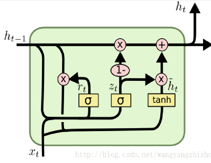
重置门
$$
r_t = \sigma(W_r \cdot [h_{t-1}, x_t] + b_r)
$$
1
|
r_t = torch.sigmoid(h @ self.W_hr + x_t @ self.W_xr + self.b_r)
|
更新门
$$
z_t = \sigma(W_z \cdot [h_{t-1}, x_t] + b_z)
$$
1
|
z_t = torch.sigmoid(h @ self.W_hz + x_t @ self.W_xz + self.b_z)
|
更新候选状态
$$
\tilde{h}t = \tanh(W_h \cdot [r_t \odot h{i-1}, x_t] + b_h)
$$
1
|
candidate_h = torch.tanh((r_t * h) @ self.W_hh + x_t @ self.W_xh + self.b_h)
|
$\tilde{h}t$为候选状态,重置门权重$r_t$决定$h{t-1}$保留多少。
更新隐藏状态
$$
h_t = (1 - z_t) \odot h_{t-1} + z_t \odot \tilde{h}_t
$$
1
|
h = (1 - z_t) * h + z_t * candidate_h
|
更新门权重$z_t$控制了最后的加权结果。如果z_t接近0,$h_t$接近于$h_{t-1}$;若接近于1,$h_t$接近于$\tilde{h}_t$。
Pytorch实现
 1
 2
 3
 4
 5
 6
 7
 8
 9
10
11
12
13
14
15
16
17
|
class GRUModel(nn.Module):
    def __init__(self, input_size, hidden_size, num_layers, output_size):
        super(GRUModel, self).__init__()
        self.hidden_size = hidden_size
        self.num_layers = num_layers
        self.gru = nn.GRU(input_size, hidden_size, num_layers, batch_first=True)
        self.fc = nn.Linear(hidden_size, output_size)

    def forward(self, x):
        # 初始化隐藏状态
        # 前向传播GRU
        out, _ = self.gru(x)
        # 从GRU的最后一层获取最后一个时间步的输出
        out = out[:, -1, :]
        # 全连接层
        out = self.fc(out)
        return out
|
 1
 2
 3
 4
 5
 6
 7
 8
 9
10
11
12
13
14
15
16
17
18
19
20
21
22
23
24
25
26
27
28
29
30
31
32
33
34
35
36
37
38
39
|
class SimpleGRU(nn.Module):
    def __init__(self, input_dim, hidden_dim, output_dim=1):
        super(SimpleGRU, self).__init__()
        self.hidden_dim = hidden_dim
        # 定义每一层的权重和偏置
        self.W_xr = nn.Parameter(torch.randn(input_dim, hidden_dim))
        self.W_hr = nn.Parameter(torch.randn(hidden_dim, hidden_dim))
        self.b_r = nn.Parameter(torch.randn(hidden_dim))

        self.W_xz = nn.Parameter(torch.randn(input_dim, hidden_dim))
        self.W_hz = nn.Parameter(torch.randn(hidden_dim, hidden_dim))
        self.b_z = nn.Parameter(torch.randn(hidden_dim))

        self.W_xh = nn.Parameter(torch.randn(input_dim, hidden_dim))
        self.W_hh = nn.Parameter(torch.randn(hidden_dim, hidden_dim))
        self.b_h = nn.Parameter(torch.randn(hidden_dim))

        # 输出层
        self.fc = nn.Linear(hidden_dim, output_dim)

    def forward(self, x):
        # x 的形状: (batch_size, sequence_length, input_dim)
        batch_size, sequence_length, input_dim = x.size()
        # 初始化隐藏状态
        h = torch.zeros(batch_size, self.hidden_dim)

        # nn.GRU相当于做了这个循环
        # 遍历时间步
        for t in range(sequence_length):
            x_t = x[:, t, :]  # 当前时间步的输入 (batch_size, input_dim)
            r_t = torch.sigmoid(h @ self.W_hr + x_t @ self.W_xr + self.b_r)
            z_t = torch.sigmoid(h @ self.W_hz + x_t @ self.W_xz + self.b_z)
            candidate_h = torch.tanh((r_t * h) @ self.W_hh + x_t @ self.W_xh + self.b_h)
            h = (1 - z_t) * h + z_t * candidate_h
            # 可以看出和公式一一对应

        # 取最后一层的最后一个时间步的隐藏状态
        output = self.fc(h)
        return output
|
经过这次实战,掌握了RNN、LSTM和GRU的深层原理。对于深度学习,有必要弄明白每个模块是干什么的,如何对应代码,这样才能有真正的提高。

